Two Disciplines, One Workflow
There is recurring confusion in engineering teams that are new to additive manufacturing: generative design and topology optimization are often treated as synonyms. They are not, and the distinction matters when you are trying to produce a printable, inspectable, cost-effective part.
Topology optimization is a mathematical process. Given a design space, load cases, constraints, and a target volume fraction, it calculates where material is structurally efficient and where it is not. The output is typically a density field — a map of material presence that tells you what to keep and what to remove.
Generative design is an engineering workflow. It uses topology optimization as a core engine, but wraps it in manufacturing constraints, material selection logic, and geometry interpretation. The output is a manufacturable geometry — or several viable geometries for different manufacturing routes.
Surface modeling is what makes the topology result usable. Raw topology output is blocky, faceted, and difficult to inspect at interfaces. Surface modeling — using T-splines, subdivision surfaces, or implicit field techniques — converts the organic topology result into smooth, printable, inspectable geometry.
The Topology Optimization Process in Detail
A well-structured topology optimization workflow has five phases:
Phase 1: Design Space Definition
The design space is the maximum envelope the part can occupy. This usually includes:
- The bounding volume of the original part
- Keep-in zones — interfaces, attachment points, assembly clearances
- Keep-out zones — adjacent components, cable routing, inspection access
# Pseudo-code: design space definition for a bracket
design_space = {
    "bounding_box": (120, 80, 45),   # mm, L×W×H
    "keep_in": [
        ("bolt_holes", [(10,10,0), (110,10,0), (10,70,0), (110,70,0)], dia=8),
        ("load_face",  (0, 0, 22.5),  area=(120, 80)),
    ],
    "keep_out": [
        ("cable_run",  (30, 20, 0),   size=(60, 40, 15)),
        ("inspection", (50, 35, 30),  size=(20, 10, 15)),
    ],
    "volume_fraction_target": 0.30,  # 30% of total design space
}
Phase 2: Load Case Definition
Multiple load cases must be defined — not just the peak load, but every significant loading scenario:
| Load Case | Magnitude | Direction | Factor |
|---|---|---|---|
| Primary load | 450 N | -Z (vertical) | 1.5× safety |
| Lateral inertia | 180 N | +X (lateral) | 2.5× (impact) |
| Thermal | ΔT = 80 °C | Uniform | 1.0× |
| Vibration base | 7.7 Grms | Z-axis | Frequency sweep |
Running optimization against a single load case is the most common mistake. Parts fail under lateral or torsional loads that were never included in the design.
Phase 3: Topology Optimization Solve
Modern solvers such as Altair OptiStruct, Autodesk Fusion, and nTopology use density-based optimization methods such as SIMP (Solid Isotropic Material with Penalization) or related approaches to converge on an efficient material distribution. Convergence often occurs in 50 to 200 iterations, depending on mesh density and constraint complexity.
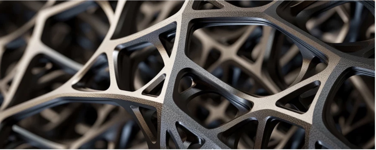
The raw result is usually a density field, an extracted iso-surface, or a triangulated mesh such as .stl that represents the material distribution. It is often described as "looking like bones." That is not accidental: bone is a biological structure that has evolved under load over millions of years.
Phase 4: Geometry Interpretation and Surface Modeling
This is where most teams underinvest. Raw topology output cannot be directly printed and inspected to GD&T tolerances. It must be interpreted into smooth, controlled geometry.
Three common approaches:
1. Manual NURBS refit — highest quality, most labor. A skilled surface modeler uses the topology result as a reference and rebuilds it as a clean NURBS surface model. Result: parameterized, inspectable, revision-friendly geometry.
2. T-spline fitting — semi-automatic. Tools such as Fusion 360 Form or Rhino-based T-spline workflows wrap a smooth surface over the topology mesh. This is faster, but surface quality can degrade at difficult intersections.
3. Implicit or field-driven geometry — the newest approach. Tools such as nTopology represent geometry as a mathematical field rather than a surface mesh. This naturally produces smooth, additive-ready geometry and handles lattice infill well.
# nTopology-style implicit field workflow (pseudo-code)
import ntopology as nt

# Load topology result
topo_field = nt.Field.from_stl("topology_result.stl")

# Smooth the field
smoothed = topo_field.smooth(iterations=5, strength=0.7)

# Convert to printable surface
surface = smoothed.isosurface(isovalue=0.5)

# Add minimum wall thickness constraint
thickened = surface.offset(min_thickness=1.5)  # mm

# Extract for printing
thickened.export("bracket_final.stl")
Phase 5: Validation
The final geometry must be validated by FEA using the actual part geometry — not the topology density field. This is a separate analysis step, and it often reveals that the interpreted surface performs slightly differently from the optimization prediction.
Typical engineering target: keep validated performance within 10–15% of the optimization prediction. If the gap is larger, the geometry interpretation usually needs refinement.
Surface Modeling Techniques for Organic Geometries
Subdivision Surfaces
Subdivision surfaces (SubD) start from a coarse control cage and subdivide recursively to produce smooth, organic geometry. Common tools include Rhino SubD, Blender, and Fusion 360 Form.
Advantages:
- Produces smooth organic surfaces quickly
- Easy to manipulate globally and locally
- Can be converted to NURBS for downstream engineering work
Disadvantages:
- Limited dimensional control compared with fully parametric CAD
- Major changes can become destructive without a clean modeling strategy
T-Splines / NURBS Hybrid
T-splines allow T-junctions that standard NURBS patches cannot represent directly. That makes it easier to cover complex organic geometry with fewer patches, trims, and visible seams. This is one reason they work well as a bridge between topology output and production CAD.
Lattice and Triply Periodic Minimal Surfaces (TPMS)
For internal structure, topology optimization often transitions into lattice design. TPMS geometries — gyroid, Schwarz P, and Diamond — provide excellent stiffness-to-weight characteristics and are inherently well suited to additive manufacturing.
# Gyroid TPMS implicit function
import numpy as np

def gyroid(x, y, z, period=5.0):
    """
    Gyroid TPMS: zero-crossing defines the surface.
    period: unit cell size in mm
    """
    p = 2 * np.pi / period
    return (
        np.sin(p * x) * np.cos(p * y) +
        np.sin(p * y) * np.cos(p * z) +
        np.sin(p * z) * np.cos(p * x)
    )

# Generate 3D field
resolution = 100
coords = np.linspace(0, 20, resolution)
X, Y, Z = np.meshgrid(coords, coords, coords)
G = gyroid(X, Y, Z, period=4.0)

# The surface is where G == 0
# Positive values = material, negative = void (or vice versa)
print(f"Volume fraction: {(G > 0).sum() / G.size * 100:.1f}%")
Gyroid infill is valued because it spreads load smoothly, avoids weak orthogonal stress paths, and prints cleanly without sharp internal corners. Exact stiffness depends on cell size, wall thickness, material, and print orientation, so it should be treated as an engineering variable rather than a universal constant.
From Simulation to Print: The Complete Workflow
At Builders Generation, our generative design workflow runs:
- Brief — load cases, interfaces, weight target, material options
- Topology solve — Altair OptiStruct or nTopology
- Geometry interpretation — NURBS or implicit surface modeling
- FEA validation — confirm target structural performance
- Printability review — support requirements, orientation, minimum features
- Print — FFF in PA-CF, PC-CF, PEEK, or ULTEM depending on application
- First article — dimensional inspection, mechanical test if required
- Delivery — with full documentation package
The turnaround from brief to printed first article is typically 7–14 days for standard engineering polymers. For PEEK and ULTEM programs, plan on 14–21 days including qualification documentation.
The geometry that topology optimization suggests and the geometry that can be manufactured are converging. With CF-PEEK in an IDEX high-temperature chamber, we can now build the organic structures that finite element methods have long indicated are efficient.